Dynare is a rich software to solve, estimate and analyse rational expectation models. While it was originally designed to solve and estimate DSGE models, Dynare has also recently been used to solve and simulate heterogeneous agents models (see Winberry and Ragot for two very different approaches). Below is a simple example on how to solve and simulate a simple RBC model using Dynare.
A simple model
The economy is composed of a representative agent who maximizes his expected
discounted sum of utility by choosing consumption $C_t$ and labor $L_t$ for $t=1,…,\infty$
$$ \sum_{t=1}^{+\infty}\big(\frac{1}{1+\rho}\big)^{t-1} E_t\Big[log(C_t)-\frac{L_t^{1+\gamma}}{1+\gamma}\Big] $$
subject to the constraint
$$ K_t = K_t{-_1} (1-\delta) + w_t L_t + r_t K_t-_1 - C_t $$
where
- $\rho \in (0,\infty)$ is the rate of time preference
- $\gamma \in (0,\infty)$ is a labor supply parameter
- $w_t$ is real wage
- $r_t$ is the real rental rate
- $K_t$ is capital at the end of the period
- $\delta \in (0,1)$ is the capital depreciation rate
The production function writes \begin{equation} Y_t = A_t K_t-_1^\alpha \Big((1+g)^t \Big)^{1-\alpha} \end{equation}
where
- $g \in (0,\infty)$ is the growth rate of production
- $\alpha$ and $\beta$ are technology parameters
- $A_t$ is a technological shock that follows and $AR(1)$ process
\begin{equation} \log(A_t) = \lambda log(A_t-_1) + e_t\end{equation}
with $e_t$ an i.i.d zero-mean normally distributed error term with standard deviation $\sigma_1$ and $\lambda \in (0,1)$ a parameter governing the persistence of shocks.
First Order conditions
The F.O.C.s of the (stationarized) model are
$$ \frac{1}{\hat{C_t}} = \frac{1}{1+\rho} E_t \Big( \frac{r_t+_1 + 1 - \delta}{\hat{C}_t+_1 (1+g)} \Big)$$
$$ L_t^\gamma = \frac{\hat{w}_t}{\hat{C}_t}$$
$$ r_t = \alpha A_t \Big(\frac{\hat{K}_t-_1}{1+g}\Big)^{\alpha-1}L_t^{1-\alpha}$$
$$ \hat{w}_t = (1-\alpha) A_t \Big(\frac{\hat{K}_t-_1}{1+g}\Big)^{\alpha}L_t^{-\alpha} $$
$$ \hat{K}_t + \hat{C}_t = \frac{\hat{K}_t-_1}{1+g} (1-\delta) + A_t \Big( \frac{\hat{K}_t-_1}{1+g} \Big)^{\alpha} L_t^{1-\alpha} $$
with $$ \hat{C}_t = \frac{C_t}{(1+g)^t}$$ $$ \hat{K}_t = \frac{K_t}{(1+g)^t}$$ $$ \hat{w}_t = \frac{w_t}{(1+g)^t}$$
Solving and simulating the model in Dynare
In Dynare, one has first to specify the endogenous variables (var), exogenous variables (varexo),
and the parameters
var C K L w r A;
varexo e;

parameters rho delta gamma alpha lambda g;
alpha = 0.33;
delta = 0.1;
rho = 0.03;
lambda = 0.97;
gamma = 0;
g = 0.015;
In a second step, the F.O.C.s of the model has to be expressed using the command model
model;
1/C=1/(1+rho)*(1/(C(+1)*(1+g)))*(r(+1)+1-delta);
L^gamma = w/C;
r = alpha*A*(K(-1)/(1+g))^(alpha-1)*L^(1-alpha);
w = (1-alpha)*A*(K(-1)/(1+g))^alpha*L^(-alpha);
K+C = (K(-1)/(1+g))*(1-delta)
+A*(K(-1)/(1+g))^alpha*L^(1-alpha);
log(A) = lambda*log(A(-1))+e;
end;
The user must provide the analytical solution for the steady state of the model using the command steady_state_model.
The command steady solves for the steady state values of the model
steady_state_model;
A = 1;
r = (1+g)*(1+rho)+delta-1;
L = ((1-alpha)/(r/alpha-delta-g))*r/alpha;
K = (1+g)*(r/alpha)^(1/(alpha-1))*L;
C = (1-delta)*K/(1+g)
+(K/(1+g))^alpha*L^(1-alpha)-K;
w = C;
end;

steady;
The command shocks defines the type of shock to be simulated
shocks;
var e; stderr 0.01;
end;

check;
A first order expansion around the steady state is obtained using the command
stoch_simul(order=1)
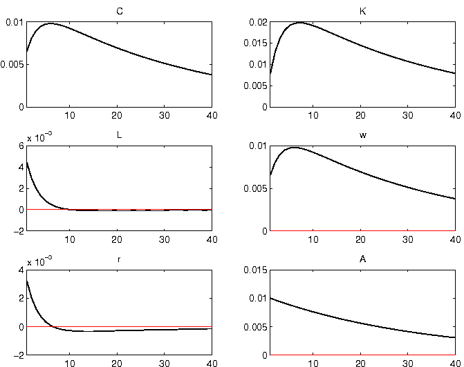
This function computes impulse response functions (IRF) and returns various descriptive statistics (moments, variance decomposition, correlation and autocorrelation coefficients)
The IRF produced by Dynare should be pretty similar to the following graph: