A Primer to Parallel Computing with Julia
With this post, my aim is to provide a non-technical introduction to parallel computing using Julia. Our goal is to calculate an approximation of $\pi$ using Monte-Carlo. I will use this example to introduce some basic Julia functions and concepts. For a more rigorous explanation, the manual is a must-read.
Calculating $\pi$ using Monte-Carlo
Our strategy to calculate an approximation of $\pi$ is quite simple. Let us consider a circle with radius $R$ inscribed in a square with side $2R$. The area of the circle, denoted by $a$, divided by the area of the square, denoted by $b$, is equal to $\frac{\pi}{4}$. Multiplying $\frac{a}{b}$ by $4$ gives us $\pi$. A slow but robust way of approximating areas is given by Monte-Carlo integration. In a nutshell, if we draw $N$ points within the square at random and we calculate the number of them falling within the circle denoted by $N_c$, $\frac{N_c}{N}$ gives us an approximation for $\frac{a}{b}$. The more draws, the more accurate the approximation.
A serial implementation
Let’s start with a serial version of the code
using Distributions
using BenchmarkTools
using Plots
using Distributed
┌ Info: Precompiling Plots [91a5bcdd-55d7-5caf-9e0b-520d859cae80]
└ @ Base loading.jl:1192
#------------------------------------------------------------
# Function that returns 1 if the point with coordinates (x,y)
# is within the unit circle; 0 otherwise
#------------------------------------------------------------
function inside_circle(x::Float64, y::Float64)
    output = 0
    if x^2 + y^2 <= 1
        output = 1
    end
    return output
end
inside_circle (generic function with 1 method)
#------------------------------------------------------------
# Function to calculate an approximation of pi
#------------------------------------------------------------
function pi_serial(nbPoints::Int64 = 128 * 1000; d=Uniform(-1.0,1.0))

   #draw NbPoints from within the square centered in 0
   #with side length equal to 2
   xDraws = rand(d, nbPoints)
   yDraws = rand(d, nbPoints)
   sumInCircle = 0

   for (xValue, yValue) in zip(xDraws, yDraws)
        sumInCircle+=inside_circle(xValue, yValue)
   end

   return 4*sumInCircle/nbPoints

end
pi_serial (generic function with 2 methods)
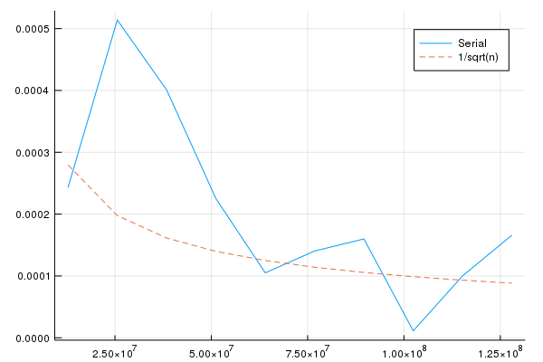
We can draw an increasing number of points and see how well the approximation for $\pi$ performs. The following figure shows that increasing the number of points leads to a smaller error, even though the decreasing pattern is not uniform. The dashed line shows that the error descreases at a rate equal to the inverse of the square root of $N$.
minPoints =  128 * 100000
maxPoints =  128 * 1000000
gridPoints = collect(minPoints:minPoints:maxPoints)
nbGridPoints = length(gridPoints)

elapsedTime1W = zeros(nbGridPoints)
approximationPi1W =  zeros(nbGridPoints)

for (index, nbDraws) in enumerate(gridPoints)

    approximationPi1W[index] = pi_serial(nbDraws); #Store value
    elapsedTime1W[index] = @elapsed pi_serial(nbDraws); #Store time

end
p = Plots.plot(gridPoints, abs.(approximationPi1W .- pi), label = "Serial")
Plots.plot!(gridPoints, 1 ./(sqrt.(gridPoints)), label = "1/sqrt(n)", linestyle = :dash)
display(p)
Plots.savefig(p, "convergence_rate.png")
Adding “workers”
When starting Julia, by default, only one processor is available. To increase the number of processors, one can use the command addprocs
println("Initial number of workers = $(nworkers())")
addprocs(4)
println("Current number of workers = $(nworkers())")
Initial number of workers = 1
Current number of workers = 4
@spawn and fetch
With Julia, one can go quite far only using the @spawnat and fetch functions.
The command @spawnat starts an operation on a given process and returns an object of type Future.
For instance, the next line starts the operation myid() on process 2:
f = @spawnat 2 myid()
Future(2, 1, 6, nothing)
To get the result from the operation we just started on process 2, we need to “fetch” the results using the Future
created above. As expected, the result is 2:
fetch(f)
2
An important thing to know about @spawnat is that the “spawning” process will not wait for the operation to be finished before moving to the next task. This can be illustrated with following example:
@time @spawnat 2 sleep(2.0)
  0.008938 seconds (11.45 k allocations: 592.538 KiB)


Future(2, 1, 8, nothing)
If the expected behavior is to wait for 2 seconds, this can be achieved by “fetching” the above operation:
@time fetch(@spawnat 2 sleep(2.0))
2.101521 seconds (47.66 k allocations: 2.357 MiB, 0.48% gc time)
The bottom line is that process 1 can be used to start many operations in parallel using @spawnat and then collects the results from the different processes using fetch.
A parallel implementation
The strategy we used to approximate $\pi$ does not need to be executed in serial. Since each draw is independent from previous ones, we could split the work between available workers (4 workers in this example). Each worker will calculate its own approximation for $\pi$ and the final result will be average value across workers.
#------------------------------------------------------------
# Let's redefine the function @everywhere so it can run on
# the newly added workers
#-----------------------------------------------------------
@everywhere function inside_circle(x::Float64, y::Float64)
    output = 0
    if x^2 + y^2 <= 1
        output = 1
    end
    return output
end
@everywhere using Distributions
#------------------------------------------------------------
# Let's redefine the function @everywhere so it can run on
# the newly added workers
#-----------------------------------------------------------
@everywhere function pi_serial(nbPoints::Int64 = 128 * 1000; d=Uniform(-1.0,1.0))

   #draw NbPoints from within the square centered in 0
   #with side length equal to 2
   xDraws = rand(d, nbPoints)
   yDraws = rand(d, nbPoints)
   sumInCircle = 0

   for (xValue, yValue) in zip(xDraws, yDraws)
        sumInCircle+=inside_circle(xValue, yValue)
   end

   return 4*sumInCircle/nbPoints

end
@everywhere function pi_parallel(nbPoints::Int64 = 128 * 1000)

   # to store different approximations
   #----------------------------------
   piWorkers = zeros(nworkers())
   # to store Futures
   #-----------------
   listFutures=[]
   # divide the draws among workers
   #-------------------------------
   nbDraws = Int(nbPoints/4)

   # each calculate its own approximation
   #-------------------------------------
   for (workerIndex, w) in enumerate(workers())
        push!(listFutures, @spawnat w pi_serial(nbDraws))
   end
   # let's fetch results
   #--------------------
   for (workerIndex, w) in enumerate(workers())
         piWorkers[workerIndex] = fetch(listFutures[workerIndex])
   end

   # return the mean value across worker
   return mean(piWorkers)

end
minPoints =  128 * 100000
maxPoints =  128 * 1000000
gridPoints = collect(minPoints:minPoints:maxPoints)
nbGridPoints = length(gridPoints)

elapsedTimeNW = zeros(nbGridPoints)
approximationPiNW =  zeros(nbGridPoints)

for (index, nbDraws) in enumerate(gridPoints)

    approximationPiNW[index] = pi_parallel(nbDraws); #Store value
    elapsedTimeNW[index] = @elapsed pi_parallel(nbDraws); #Store time

end
Serial vs parallel comparisons
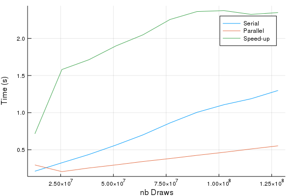
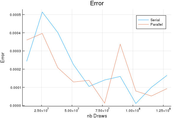
In terms of accuracy, the serial and the parallel codes generate the same results (modulo randomness). In terms of speed, the parallel version is up to 2.5 times faster. The more points are drawn, the higher the speed-gains. This example shows the well-established fact that the advantages of parallel computing start to kick-in when the underlying tasks are time-consuming in the first place.
p = Plots.plot(gridPoints, abs.(approximationPi1W .- pi), label = "Serial")
Plots.plot!(gridPoints, abs.(approximationPiNW .- pi), label = "Parallel")
Plots.title!("Error")
Plots.xlabel!("nb Draws")
Plots.ylabel!("Error")
display(p)
Plots.savefig(p,"error_comparison.png")
p = Plots.plot(gridPoints, elapsedTime1W, label = "Serial")
Plots.plot!(gridPoints, elapsedTimeNW, label = "Parallel")
Plots.plot!(gridPoints, elapsedTime1W./elapsedTimeNW, label = "Speed-up")
Plots.xlabel!("nb Draws")
Plots.ylabel!("Time (s)")
display(p)
Plots.savefig("Speed_gains.png")