A large class of economic models involves solving for functional equations of the form:

A well known example is the stochastic optimal growth model. An agent owns a consumption good $y$ at time $t$, which can be consumed or invested. Next period’s output depends on how much is invested at time $t$ and on a shock $z$ realized at the end of the current period. One can think of a farmer deciding the quantity of seeds to be planted during the spring, taking into account weather forecast for the growing season.
A common technique for solving this class of problem is value function iteration. While value function iteration is quite intuitive, it is not the only one available. In this post, I describe the collocation method, which transforms the problem of finding a function into a problem of finding a vector that satisfies a given set of conditions. The gain from this change of perspective is that any root-finding algorithm can then be used. In particular, one may use the Newton method, which converges at a quadratic rate in the neighborhood of the solution if the function is smooth enough.
Value function iteration
Value function iteration takes advantage of the fact that the Bellman operator $T$ is a contraction mapping on the set of continuous bounded functions on $\mathbb R_+$ under the supremum distance
 An immediate consequence if that the sequence $w,Tw,T^2w$,… converges uniformly to $w$ (starting with any bounded and continuous function $w$). The following code in
 Julia v0.6.4 illustrates the convergence of the series ${T^nw}$.
 #=
Julien Pascal
Code heavily based on:
----------------------
https://lectures.quantecon.org/jl/optgrowth.html
by Spencer Lyon, John Stachurski
I have only made minor modifications:
#------------------------------------
* I added a type optGrowth
* I use the package Interpolations
* I calculate the expectation w.r.t the aggregate
  shock using a Gauss-Legendre quadrature scheme
  instead of Monte-Carlo
=#

using QuantEcon
using Optim
using CompEcon
using PyPlot
using Interpolations
using FileIO


type optGrowth

  w::Array{Float64,1}
  β::AbstractFloat
  grid::Array{Float64,1}
  u::Function
  f::Function
  shocks::Array{Float64,1}
  Tw::Array{Float64,1}
  σ::Array{Float64,1}
  el_k::Array{Float64,1}
  wl_k::Array{Float64,1}
  compute_policy::Bool
  w_func::Function

end

function optGrowth(;w = Array{Float64,1}[],
                    α = 0.4,
                    β = 0.96,
                    μ = 0,
                    s = 0.1,
                    grid_max = 4,         # Largest grid point
                    grid_size = 200,      # Number of grid points
                    shock_size = 250,     # Number of shock draws in Monte Carlo integral
                    Tw = Array{Float64,1}[],
                    σ = Array{Float64,1}[],
                    el_k = Array{Float64,1}[],
                    wl_k = Array{Float64,1}[],
                    compute_policy = true
                  )


  grid_y = collect(linspace(1e-5, grid_max, grid_size))
  shocks = exp.(μ + s * randn(shock_size))

  # Utility
  u(c) = log(c)
  # Production
  f(k) = k^α

  w = 5 * log.(grid_y)
  Tw = 5 * log.(grid_y)
  σ = 5 * log.(grid_y)

  el_k, wl_k = qnwlogn(10, μ, s^2) #10 weights and nodes for LOG(e_t) distributed N(μ,s^2)

  w_func = x -> x
  optGrowth(
    w,
    β,
    grid_y,
    u,
    f,
    shocks,
    Tw,
    σ,
    el_k,
    wl_k,
    compute_policy,
    w_func
    )
end

"""
The approximate Bellman operator, which computes and returns the
updated value function Tw on the grid points.
#### Arguments
`model` : a model of type optGrowth
`Modifies model.σ, model.w and model.Tw
"""
function bellman_operator!(model::optGrowth)

    # === Apply linear interpolation to w === #
    knots = (model.grid,)
    itp = interpolate(knots, model.w, Gridded(Linear()))

    #w_func(x) = itp[x]

    model.w_func = x -> itp[x]

    if model.compute_policy
        model.σ = similar(model.w)
    end

    # == set Tw[i] = max_c { u(c) + β E w(f(y  - c) z)} == #
    for (i, y) in enumerate(model.grid)

        #Monte Carlo
        #-----------
        #objective(c) = - model.u(c) - model.β * mean(w_func(model.f(y - c) .* model.shocks))

        #Gauss-Legendre
        #--------------
        function objective(c)

          expectation = 0.0

          for k = 1:length(model.wl_k)
            expectation += model.wl_k[k]*(model.w_func(model.f(y - c) * model.el_k[k]))
          end

          - model.u(c) - model.β * expectation

        end

        res = optimize(objective, 1e-10, y)

        if model.compute_policy
            model.σ[i] = Optim.minimizer(res)
        end

        model.Tw[i] = - Optim.minimum(res)
        model.w[i] = - Optim.minimum(res)
    end


end


model = optGrowth()

function solve_optgrowth!(model::optGrowth;
                         tol::AbstractFloat=1e-6,
                         max_iter::Integer=500)

    w_old = copy(model.w)  # Set initial condition
    error = tol + 1
    i = 0


    # Iterate to find solution
    while i < max_iter

        #update model.w
        bellman_operator!(model)
        error = maximum(abs, model.w - w_old)

        if error < tol
          break
        end

        w_old = copy(model.w)
        i += 1
    end

end

#-----------------------------------
# Solve by value function iteration
#-----------------------------------
@time solve_optgrowth!(model)
# 3.230501 seconds (118.18 M allocations: 1.776 GiB, 3.51% gc time)


#-------------------------------
# Compare with the true solution
#-------------------------------
α = 0.4
β = 0.96
μ = 0
s = 0.1

c1 = log(1 - α * β) / (1 - β)
c2 = (μ + α * log(α * β)) / (1 - α)
c3 = 1 / (1 - β)
c4 = 1 / (1 - α * β)


# True optimal policy
c_star(y) = (1 - α * β) * y

# True value function
v_star(y) = c1 + c2 * (c3 - c4) + c4 * log.(y)

fig, ax = subplots(figsize=(9, 5))
ax[:set_ylim](-35, -24)
ax[:plot](model.grid, model.w_func.(model.grid), lw=2, alpha=0.6, label="Approximated (VFI)", linestyle="--")
ax[:plot](model.grid, v_star.(model.grid), lw=2, alpha=0.6, label="Exact value")
ax[:legend](loc="lower right")
savefig("value_function_iteration.png")

fig, ax = subplots(figsize=(9, 5))
ax[:set_xlim](0.1, 4.0)
ax[:set_ylim](0.00, 0.008)
ax[:plot](model.grid, abs.(model.w_func.(model.grid) -v_star.(model.grid)), lw=2, alpha=0.6, label="error")
ax[:legend](loc="lower right")
savefig("error_value_function_iteration.png")
Output
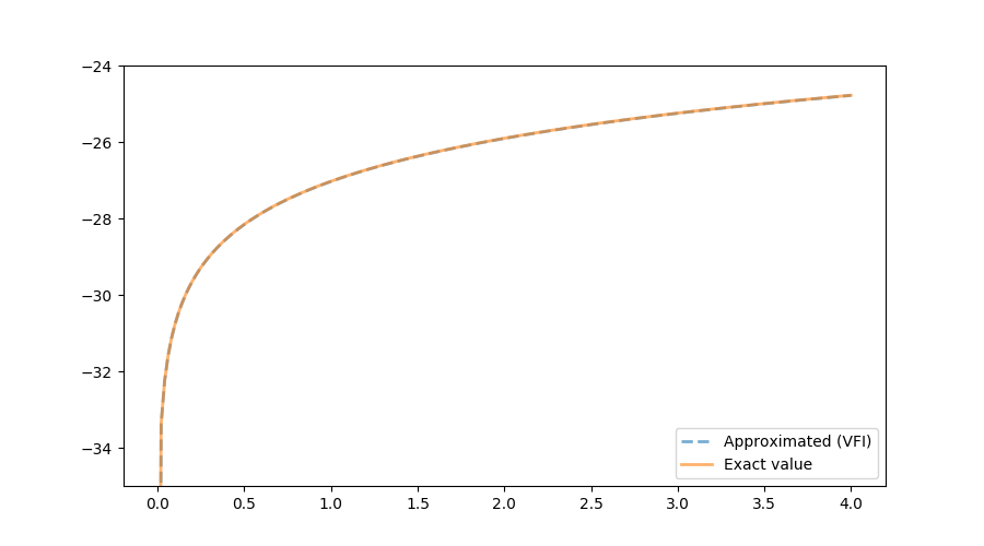
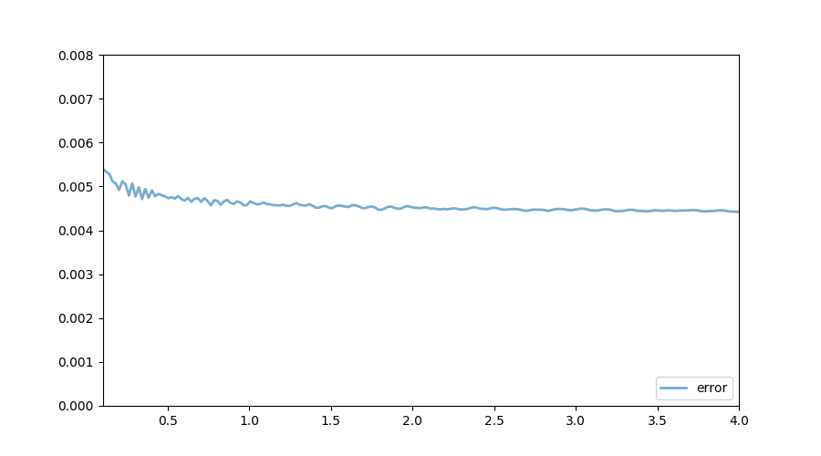
The following figure shows the exact function, which we know in this very specific case, and the one calculated using VFI. Both quantities are almost indistinguishable. As the illustrated in the next figure, the (absolute value) of the distance between the true and the approximated values is bounded above by $0.006$. The accuracy of the current approximation could be improved by iterating the process further.
The collocation method
The collocation method takes a different route. Let us remember that we are looking for a function $w$. Instead of solving for the values of $w$ on a grid and then interpolating, why not looking for a function directly? To do so, let us assume that $w$ can reasonably be approximated by a function $\hat{w}$:
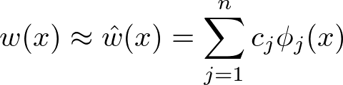
with $ \phi_1(x) $ , $ \phi_2(x) $,…, $ \phi_n(x) $ a set of linearly independent basis functions and $c_1$, $c_2$, …, $c_n$ $n$ coefficient to be found. Replacing $w(x)$ with $\hat{w(x)}$ into the functional equation and reorganizing gives:
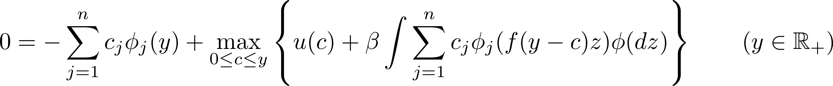
This equation has to hold (almost) exactly at $n$ points (also called nodes): $y_1$, $y_2$, …, $y_n$:

The equation above defines a system of $n$ equation with as many unknown, which can be compactly written as: $$ f(\boldsymbol{c}) = \boldsymbol{0} $$
Newton or quasi-Newton can be used to solve for the root of $f$. In the code that follows, I use Broyden’s method. Let us illustrate this technique using a Chebychev polynomial basis and Chebychev nodes. In doing so, we avoid Runge’s phenomenon associated with a uniform grid.
Implementation using CompEcon
#---------------------------------------------
# Julien Pascal
# Solve the stochastic optimal growth problem
# using the collocation method
#---------------------------------------------
using QuantEcon
using Optim
using CompEcon
using PyPlot
using Interpolations
type optGrowthCollocation
w::Array{Float64,1}
β::AbstractFloat
grid::Array{Float64,1}
u::Function
f::Function
shocks::Array{Float64,1}
Tw::Array{Float64,1}
σ::Array{Float64,1}
el_k::Array{Float64,1}
wl_k::Array{Float64,1}
compute_policy::Bool
order_approximation::Int64 #number of element in the functional basis along each dimension
functional_basis_type::String #type of functional basis
fspace::Dict{Symbol,Any} #functional basis
fnodes::Array{Float64,1} #collocation nodes
residual::Array{Float64,1} #vector of residual. Should be close to zero
a::Array{Float64,1} #polynomial coefficients
w_func::Function
end
#####################################
# Function that finds a solution
# to f(x) = 0
# using Broyden's "good" method
# and a simple backstepping procedure as described
# in Miranda and Fackler (2009)
#
# input :
# --------
# * x0: initial guess for the root
# * f: function in f(x) = 0
# * maxit: maximum number of iterations
# * tol: tolerance level for the zero
# * fjavinc: initial inverse of the jacobian. If not provided, then inverse of the
# Jacobian is calculated by finite differences
# * maxsteps: maximum number of backsteps
# * recaculateJacobian: number of iterations in-between two calculations of the Jacobian
#
# output :
# --------
# * x: one zero of f
# * it: number of iterations necessary to reached the solution
# * fjacinv: pseudo jacobian at the last iteration
# * fnorm: norm f(x) at the last iteration
#
#######################################
function find_broyden(x0::Vector, f::Function, maxit::Int64, tol::Float64, fjacinv = eye(length(x0));
maxsteps = 5, recaculateJacobian = 1)
println("a0 = $(x0)")
fnorm = tol*2
it2 = 0 #to re-initialize the jacobian
################################
#initialize guess for the matrix
################################
fjacinv_function = x-> Calculus.finite_difference_jacobian(f, x)
#fjacinv_function = x -> ForwardDiff.gradient(f, x)
# If the user do not provide an initial guess for the jacobian
# One is calculated using finite differences.
if fjacinv == eye(length(x0))
################################################
# finite differences to approximate the Jacobian
# at the initial value
# this is slow. Seems to improve performances
# when x0 is of high dimension.
println("Calculating the Jacobian by finite differences")
#@time fjacinv = Calculus.finite_difference_jacobian(f, x0)
@time fjacinv = fjacinv_function(x0)
println("Inverting the Jacobian")
try
fjacinv = inv(fjacinv)
catch
try
println("Jacobian non-invertible\n calculating pseudo-inverse")
fjacinv = pinv(A)
catch
println("Failing Calculating the pseudo-inverse. Initializing with In")
fjacinv = eye(length(x0))
end
end
println("Done")
else
println("Using User's input as a guess for the Jacobian.")
end
fval = f(x0)
for it=1:maxit
it2 +=1
#every 30 iterations, reinitilize the jacobian
if mod(it2, recaculateJacobian) == 0
println("Re-calculating the Jacobian")
fjacinv = fjacinv_function(x0)
try
fjacinv = inv(fjacinv)
catch
try
println("Jacobian non-invertible\n calculating pseudo-inverse")
fjacinv = pinv(A)
catch
println("Failing Calculating the pseudo-inverse. Initializing with In")
fjacinv = eye(length(x0))
end
end
end
println("it = $(it)")
fnorm = norm(fval)
if fnorm < tol
println("fnorm = $(fnorm)")
return x0, it, fjacinv, fnorm
end
d = -(fjacinv*fval)
fnormold = Inf
########################
# Backstepping procedure
########################
for backstep = 1:maxsteps
if backstep > 1
println("backstep = $(backstep-1)")
end
fvalnew = f(x0 + d)
fnormnew = norm(fvalnew)
if fnormnew < fnorm
break
end
if fnormold < fnormnew
d=2*d
break
end
fnormold = fnormnew
d = d/2
end
####################
####################
x0 = x0 + d
fold = fval
fval = f(x0)
u = fjacinv*(fval - fold)
#Update the pseudo Jacobian:
fjacinv = fjacinv + ((d-u)*(transpose(d)*fjacinv))/(dot(d,u))
println("a$(it) = $(x0)")
println("fnorm = $(fnorm)")
if isnan.(x0) == trues(length(x0))
println("Error. a$(it) = NaN for each component")
x0 = zeros(length(x0))
return x0, it, fjacinv, fnorm
end
end
println("In function find_broyden\n")
println("Maximum number of iterations reached.\n")
println("No convergence.")
println("Returning fnorm = NaN as a solution")
fnorm = NaN
return x0, maxit, fjacinv, fnorm
end
function optGrowthCollocation(;w = Array{Float64,1}[],
α = 0.4,
β = 0.96,
μ = 0,
s = 0.1,
grid_max = 4, # Largest grid point
grid_size = 200, # Number of grid points
shock_size = 250, # Number of shock draws in Monte Carlo integral
Tw = Array{Float64,1}[],
σ = Array{Float64,1}[],
el_k = Array{Float64,1}[],
wl_k = Array{Float64,1}[],
compute_policy = true,
order_approximation = 40,
functional_basis_type = "chebychev",
)
grid_y = collect(linspace(1e-5, grid_max, grid_size))
shocks = exp.(μ + s * randn(shock_size))
# Utility
u(c) = log.(c)
# Production
f(k) = k^α
el_k, wl_k = qnwlogn(10, μ, s^2) #10 weights and nodes for LOG(e_t) distributed N(μ,s^2)
lower_bound_support = minimum(grid_y)
upper_bound_support = maximum(grid_y)
n_functional_basis = [order_approximation]
if functional_basis_type == "chebychev"
fspace = fundefn(:cheb, n_functional_basis, lower_bound_support, upper_bound_support)
elseif functional_basis_type == "splines"
fspace = fundefn(:spli, n_functional_basis, lower_bound_support, upper_bound_support, 1)
elseif functional_basis_type == "linear"
fspace = fundefn(:lin, n_functional_basis, lower_bound_support, upper_bound_support)
else
error("functional_basis_type has to be either chebychev, splines or linear.")
end
fnodes = funnode(fspace)[1]
residual = zeros(size(fnodes)[1])
a = ones(size(fnodes)[1])
w = ones(size(fnodes)[1])
Tw = ones(size(fnodes)[1])
σ = ones(size(fnodes)[1])
w_func = x-> x
optGrowthCollocation(
w,
β,
grid_y,
u,
f,
shocks,
Tw,
σ,
el_k,
wl_k,
compute_policy,
order_approximation,
functional_basis_type,
fspace,
fnodes,
residual,
a,
w_func
)
end
function residual!(model::optGrowthCollocation)
model.w_func = y -> funeval(model.a, model.fspace, [y])[1][1]
function objective(c, y)
expectation = 0.0
for k = 1:length(model.wl_k)
expectation += model.wl_k[k]*(model.w_func(model.f(y - c) * model.el_k[k]))
end
- model.u(c) - model.β * expectation
end
# Loop over nodes
for i in 1:size(model.fnodes)[1]
y = model.fnodes[i,1]
res = optimize(c -> objective(c, y), 1e-10, y)
if model.compute_policy
model.σ[i] = Optim.minimizer(res)
end
model.Tw[i] = - Optim.minimum(res)
model.w[i] = model.w_func(y)
model.residual[i] = - model.w[i] + model.Tw[i]
end
end
model = optGrowthCollocation(functional_basis_type = "chebychev")
residual!(model)
function solve_optgrowth!(model::optGrowthCollocation;
tol=1e-6,
max_iter=500)
# Initialize guess for coefficients
# by giving the "right shape"
# ---------------------------------
function objective_initialize!(x, model)
#update polynomial coeffficients
model.a = copy(x)
model.w_func = y -> funeval(model.a, model.fspace, [y])[1][1]
return abs.(model.w_func.(model.fnodes[:,1]) - 5.0 * log.(model.fnodes[:,1]))
end
minx, iterations, Jac0, fnorm = find_broyden(model.a, x -> objective_initialize!(x, model), max_iter, tol)
# Solving the model by collocation
# using the initial guess calculated above
#-----------------------------------------
function objective_residual!(x, model)
#update polynomial coeffficients
model.a = copy(x)
#calculate residual
residual!(model)
return abs.(model.residual)
end
minx, iterations, Jac, fnorm = find_broyden(model.a, x -> objective_residual!(x, model), max_iter, tol)
end
#-----------------------------------
# Solve by collocation
#-----------------------------------
@time solve_optgrowth!(model)
#-------------------------------
# Compare with the true solution
#-------------------------------
α = 0.4
β = 0.96
μ = 0
s = 0.1
c1 = log(1 - α * β) / (1 - β)
c2 = (μ + α * log(α * β)) / (1 - α)
c3 = 1 / (1 - β)
c4 = 1 / (1 - α * β)
# True optimal policy
c_star(y) = (1 - α * β) * y
# True value function
v_star(y) = c1 + c2 * (c3 - c4) + c4 * log.(y)
fig, ax = subplots(figsize=(9, 5))
ax[:set_ylim](-35, -24)
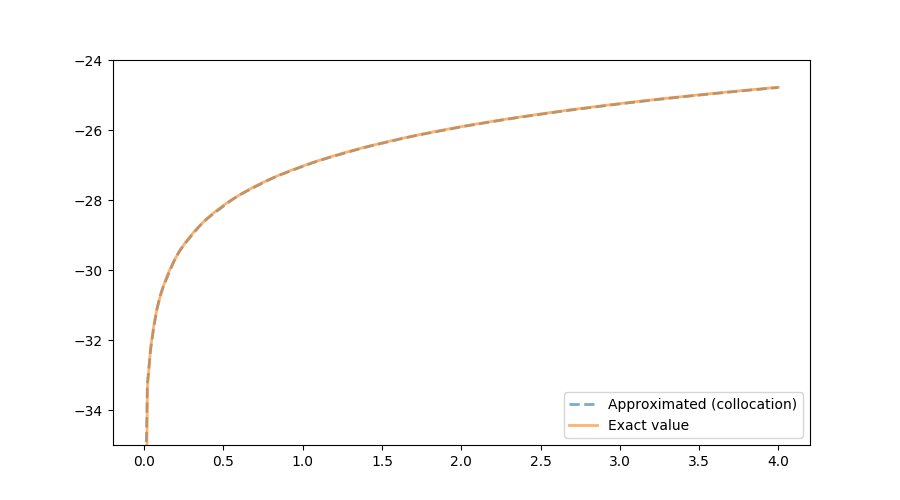
ax[:plot](model.grid, model.w_func.(model.grid), lw=2, alpha=0.6, label="Approximated (collocation)", linestyle = "--")
ax[:plot](model.grid, v_star.(model.grid), lw=2, alpha=0.6, label="Exact value")
ax[:legend](loc="lower right")
savefig("collocation.png")
fig, ax = subplots(figsize=(9, 5))
ax[:set_xlim](0.1, 4.0)
ax[:set_ylim](-0.05, 0.05)
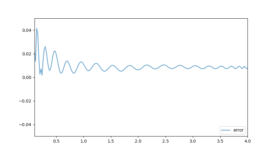
ax[:plot](model.grid, abs.(model.w_func.(model.grid) -v_star.(model.grid)), lw=2, alpha=0.6, label="error")
ax[:legend](loc="lower right")
savefig("error_collocation.png")
Output
The following figure shows the exact function and the one calculated using the collocation method. In terms of accuracy, both VFI and the collocation method generate reliable results.
In terms of speed, it turns out that the value function iteration implementation is much faster. One reason seems to be the efficiency associated with the package Interpolations: it is more than 20 times faster to evaluate $w$ using the package Interpolations rather than using the package CompEcon:
  #using Interpolations
  #--------------------
  @time for i=1:1000000
   model.w_func.(model.grid[1])
  end
  #0.230861 seconds (2.00 M allocations: 30.518 MiB, 1.28% gc time)

  #using CompEcon
  #--------------
  @time for i=1:1000000
   model.w_func.(model.grid[1])
  end
  # 4.998902 seconds (51.00 M allocations: 3.546 GiB, 13.39% gc time)
Implementation using ApproxFun
Significant speed-gains can be obtained by using the package ApproxFun, as illustrated by the code below. Computing time is divided by approximately $5$ compared to the implementation using CompEcon. Yet, the value function iteration implementation is still the fastest one. One bottleneck seems to be the calculation of the Jacobian by finite differences when using Broyden’s method. It is likely that using automatic differentiation would further improve results.
#---------------------------------------------
# Julien Pascal
# Solve the stochastic optimal growth problem
# using the collocation method
# Implementation using ApproxFun
#---------------------------------------------
using QuantEcon
using Optim
using CompEcon
using PyPlot
using Interpolations
using FileIO
using ApproxFun
using ProfileView


type optGrowthCollocation

  w::Array{Float64,1}
  β::AbstractFloat
  grid::Array{Float64,1}
  u::Function
  f::Function
  shocks::Array{Float64,1}
  Tw::Array{Float64,1}
  σ::Array{Float64,1}
  el_k::Array{Float64,1}
  wl_k::Array{Float64,1}
  compute_policy::Bool
  order_approximation::Int64 #number of element in the functional basis along each dimension
  functional_basis_type::String #type of functional basis
  fspace::Dict{Symbol,Any} #functional basis
  fnodes::Array{Float64,1} #collocation nodes
  residual::Array{Float64,1} #vector of residual. Should be close to zero
  a::Array{Float64,1} #polynomial coefficients
  fApprox::ApproxFun.Fun{ApproxFun.Chebyshev{ApproxFun.Segment{Float64},Float64},Float64,Array{Float64,1}}
  w_func::Function
  tol::Float64

end


  #####################################
  # Function that find a solution
  # to f(x) = 0
  # using Broyden's "good" method
  # and simple backstepping procedure as described
  # in Miranda and Fackler (2009)
  #
  # input :
  # --------
  # * x0:                 initial guess for the root
  # * f:                  function in f(x) = 0
  # * maxit:              maximum number of iterations
  # * tol:                tolerance level for the zero
  # * fjavinc:            initial inverse of the jacobian. If not provided, then inverse of the
  #                       Jacobian is calculated by finite differences
  # * maxsteps:           maximum number of backsteps
  # * recaculateJacobian: number of iterations in-between two calculations of the Jacobian
  #
  # output :
  # --------
  # * x: one zero of f
  # * it: number of iterations necessary to reached the solution
  # * fjacinv: pseudo jacobian at the last iteration
  # * fnorm: norm f(x) at the last iteration
  #
  #######################################
  function find_broyden(x0::Vector, f::Function, maxit::Int64, tol::Float64, fjacinv = eye(length(x0));
                        maxsteps = 5, recaculateJacobian = 1)

      println("a0 = $(x0)")
      fnorm = tol*2
      it2 = 0 #to re-initialize the jacobian

      ################################
      #initialize guess for the matrix
      ################################
      # with Calculus
      #--------------
      fjacinv_function = x-> Calculus.finite_difference_jacobian(f, x)


      # If the user do not provide an initial guess for the jacobian
      # One is calculated using finite differences.
      if fjacinv == eye(length(x0))
          ################################################
          # finite differences to approximate the Jacobian
          # at the initial value
          # this is slow. Seems to improve performances
          # when x0 is of high dimension.
          println("Calculating the Jacobian by finite differences")
          #@time fjacinv = Calculus.finite_difference_jacobian(f, x0)
          @time fjacinv = fjacinv_function(x0)

          println("Inverting the Jacobian")
          try
              fjacinv = inv(fjacinv)
          catch
              try
                  println("Jacobian non-invertible\n calculating pseudo-inverse")
                  fjacinv = pinv(A)
              catch
                  println("Failing Calculating the pseudo-inverse. Initializing with In")
                  fjacinv = eye(length(x0))
              end
          end
          println("Done")
      else
          println("Using User's input as a guess for the Jacobian.")
      end

      fval = f(x0)

      for it=1:maxit

          it2 +=1

          #every 30 iterations, reinitilize the jacobian
          if mod(it2, recaculateJacobian) == 0

              println("Re-calculating the Jacobian")

              fjacinv = fjacinv_function(x0)

              try
                  fjacinv = inv(fjacinv)
              catch
                  try
                      println("Jacobian non-invertible\n calculating pseudo-inverse")
                      fjacinv = pinv(A)
                  catch
                      println("Failing Calculating the pseudo-inverse. Initializing with In")
                      fjacinv = eye(length(x0))
                  end
              end

          end


          println("it = $(it)")

          fnorm = norm(fval)

          if fnorm < tol
              println("fnorm = $(fnorm)")
              return x0, it, fjacinv, fnorm
          end

          d = -(fjacinv*fval)

          fnormold = Inf
          ########################
          # Backstepping procedure
          ########################
          for backstep = 1:maxsteps

              if backstep > 1
                  println("backstep = $(backstep-1)")
              end

              fvalnew = f(x0 + d)
              fnormnew = norm(fvalnew)

              if fnormnew < fnorm
                  break
              end

              if fnormold < fnormnew
                  d=2*d
                  break
              end

              fnormold = fnormnew

              d = d/2

          end
          ####################
          ####################

          x0 = x0 + d

          fold = fval
          fval = f(x0)

          u = fjacinv*(fval - fold)

          #Update the pseudo Jacobian:
          fjacinv = fjacinv + ((d-u)*(transpose(d)*fjacinv))/(dot(d,u))

          println("a$(it) = $(x0)")
          println("fnorm = $(fnorm)")

          if isnan.(x0) == trues(length(x0))
              println("Error. a$(it) = NaN for each component")
              x0 = zeros(length(x0))
              return x0, it, fjacinv, fnorm
          end
      end

      println("In function find_broyden\n")
      println("Maximum number of iterations reached.\n")
      println("No convergence.")
      println("Returning fnorm = NaN as a solution")
      fnorm = NaN
      return x0, maxit, fjacinv, fnorm

  end

function optGrowthCollocation(;w = Array{Float64,1}[],
                              α = 0.4,
                              β = 0.96,
                              μ = 0,
                              s = 0.1,
                              grid_max = 4,         # Largest grid point
                              grid_size = 200,      # Number of grid points
                              shock_size = 250,     # Number of shock draws in Monte Carlo integral
                              Tw = Array{Float64,1}[],
                              σ = Array{Float64,1}[],
                              el_k = Array{Float64,1}[],
                              wl_k = Array{Float64,1}[],
                              compute_policy = true,
                              order_approximation = 40,
                              functional_basis_type = "chebychev",
                            )


  grid_y = collect(linspace(1e-4, grid_max, grid_size))
  shocks = exp.(μ + s * randn(shock_size))

  # Utility
  u(c) = log.(c)
  # Production
  f(k) = k^α

  el_k, wl_k = qnwlogn(10, μ, s^2) #10 weights and nodes for LOG(e_t) distributed N(μ,s^2)

  lower_bound_support = minimum(grid_y)
  upper_bound_support = maximum(grid_y)

  n_functional_basis = [order_approximation]

  if functional_basis_type == "chebychev"
      fspace = fundefn(:cheb, n_functional_basis, lower_bound_support, upper_bound_support)
  else
      error("functional_basis_type has to be \"chebychev\" ")
  end


  fnodes = funnode(fspace)[1]
  residual = zeros(size(fnodes)[1])
  a = ones(size(fnodes)[1])

  tol = 0.001

  fApprox = (Fun(Chebyshev((minimum(grid_y))..(maximum(grid_y))), a))
  #fApprox = (Fun(Chebyshev(0..maximum(model.grid)), a))

  w_func = x-> fApprox(x)

  w = ones(size(fnodes)[1])
  Tw = ones(size(fnodes)[1])
  σ = ones(size(fnodes)[1])


  optGrowthCollocation(
    w,
    β,
    grid_y,
    u,
    f,
    shocks,
    Tw,
    σ,
    el_k,
    wl_k,
    compute_policy,
    order_approximation,
    functional_basis_type,
    fspace,
    fnodes,
    residual,
    a,
    fApprox,
    w_func,
    tol
    )
end


function residual!(model::optGrowthCollocation)


    model.fApprox = (Fun(Chebyshev((minimum(model.grid))..(maximum(model.grid))), model.a))
    model.w_func = x-> model.fApprox(x)

    function objective(c, y)

      expectation = 0.0

      for k = 1:length(model.wl_k)
        expectation += model.wl_k[k]*(model.w_func(model.f(y - c) * model.el_k[k]))
      end

      - model.u(c) - model.β * expectation

    end

    # Loop over nodes
    for i in 1:size(model.fnodes)[1]

        y = model.fnodes[i,1]

        res = optimize(c -> objective(c, y), 1e-10, y)

        if model.compute_policy
            model.σ[i] = Optim.minimizer(res)
        end

        model.Tw[i] = - Optim.minimum(res)
        model.w[i] = model.w_func(y)

        model.residual[i] = - model.w[i] + model.Tw[i]
    end

end


function solve_optgrowth!(model::optGrowthCollocation;
                         tol=1e-6,
                         max_iter=500)

    # Initialize guess for coefficients
    # by giving the "right shape"
    # ---------------------------------
    function objective_initialize!(x, model)

      #update polynomial coeffficients
      model.a = copy(x)

      model.fApprox = (Fun(Chebyshev((minimum(model.grid))..(maximum(model.grid))), model.a))

      model.w_func = x-> model.fApprox(x)

      return abs.(model.w_func.(model.fnodes[:,1]) - 5.0 * log.(model.fnodes[:,1]))

    end


    minx, iterations, Jac0, fnorm = find_broyden(model.a, x -> objective_initialize!(x, model), max_iter, tol)


    # Solving the model by collocation
    # using the initial guess calculated above
    #-----------------------------------------
    function objective_residual!(x, model)

      #update polynomial coeffficients
      model.a = copy(x)

      #calculate residual
      residual!(model)

      return abs.(model.residual)

    end

    minx, iterations, Jac, fnorm = find_broyden(model.a, x -> objective_residual!(x, model), max_iter, tol,  recaculateJacobian = 1)


end

#-----------------------------------
# Solve by collocation
#-----------------------------------
model = optGrowthCollocation(functional_basis_type = "chebychev")
@time solve_optgrowth!(model)
# 15.865923 seconds (329.12 M allocations: 4.977 GiB, 5.55% gc time)


#-------------------------------
# Compare with the true solution
#-------------------------------
α = 0.4
β = 0.96
μ = 0
s = 0.1

c1 = log(1 - α * β) / (1 - β)
c2 = (μ + α * log(α * β)) / (1 - α)
c3 = 1 / (1 - β)
c4 = 1 / (1 - α * β)


# True optimal policy
c_star(y) = (1 - α * β) * y

# True value function
v_star(y) = c1 + c2 * (c3 - c4) + c4 * log.(y)

fig, ax = subplots(figsize=(9, 5))
ax[:set_ylim](-35, -24)
ax[:plot](model.grid, model.w_func.(model.grid), lw=2, alpha=0.6, label="approximate value function")
ax[:plot](model.grid, v_star.(model.grid), lw=2, alpha=0.6, label="true value function")

fig, ax = subplots(figsize=(9, 5))
ax[:set_xlim](0.1, 4.0)
ax[:set_ylim](- 0.05, 0.05)
ax[:plot](model.grid, abs.(model.w_func.(model.grid) -v_star.(model.grid)), lw=2, alpha=0.6, label="error")
ax[:legend](loc="lower right")